Lecture notes on Reinforcement Learning

I recently took David Silver’s online class on reinforcement learning (syllabus & slides and video lectures) to get a more solid understanding of his work at DeepMind on AlphaZero (paper and more explanatory blog post) etc. I enjoyed it as a very accessible yet practical introduction to RL. Here are the notes I took during the class.

David Silver in action

Slide numbers refer to the downloadbale slides (might differ slightly from those in the videos), and therein to the page number in parantheses (like e.g. “15” for “[15 of 47]”).

Lecture 1: Introduction to Reinforcement Learning

The RL Problem:
- RL Hypothesis: all goal achievement can be cast as maximizing cumulative future reward (“all goals can be described by maximizing expected cumulative reward”)
- History (times series of all actions/rewards/observations until now) is impractical for decision making (if the agent has a long life) -> use state instead as a condensed form of all that matters: s_t=f(H_t)
- When we talk state, we mean the agent’s state (where we can control the function f), not the environment state (invisible to us, may contain other agents)
- Our state (Information State) has to have the Markov property: future is independent of the past given the present (env. state is, complete history is too)
- Great example for how our decision depends on the choice of state: rat & cheese/electricity (order or count as state representation) -> see slide 25
- If the environment is fully obserable (obervation = environment state = agent state), the decision process is a MDP
- For partially observable environments: POMDP -> have to build our own state representation (e.g., Bayesian: have a vector of beliefs/probabilities of what state the environment is in; ML: have a RNN combine the last state and latest observation into a new state)
The pieces of a solution:
- An agent may include one or more of these: policy (behaviour function [a,s]->[s’]), value function (predicted [discounted] future reward, depending on some behaviour), model (predict what the environment will do next)
- V: State-value function; Q: Action-value function
- Transition model: predicts environment dynamics; Reward model: predicts next immediate reward
- Good example for policy/value function/model: simple maze with numbers/arrows -> see slides 35-37
- Taxonomy: value-based (policy implicit); policy-based (value function implicit); actor-critic (stores both policy and value function)
- Taxonomy contd.: model-free (policy and/or value function); model-based: has a model and policy/value function
Problems in RL:
- RL: env. initially unknown, agent has to interact to find good policy
- Planning: model of env. is known; agent performs computations with model to look ahead and choose policy (e.g., tree-search)
- Both are intimately linked, e.g. learn how env. works first (i.e., build model) and then do planning
- Exploration / exploitation: e.g. go to your favourite / a new restaurant
- Prediction / control: predict future given policy (find value function) vs. optimise future (find policy) -> usually we need to solve prediction to optimally control

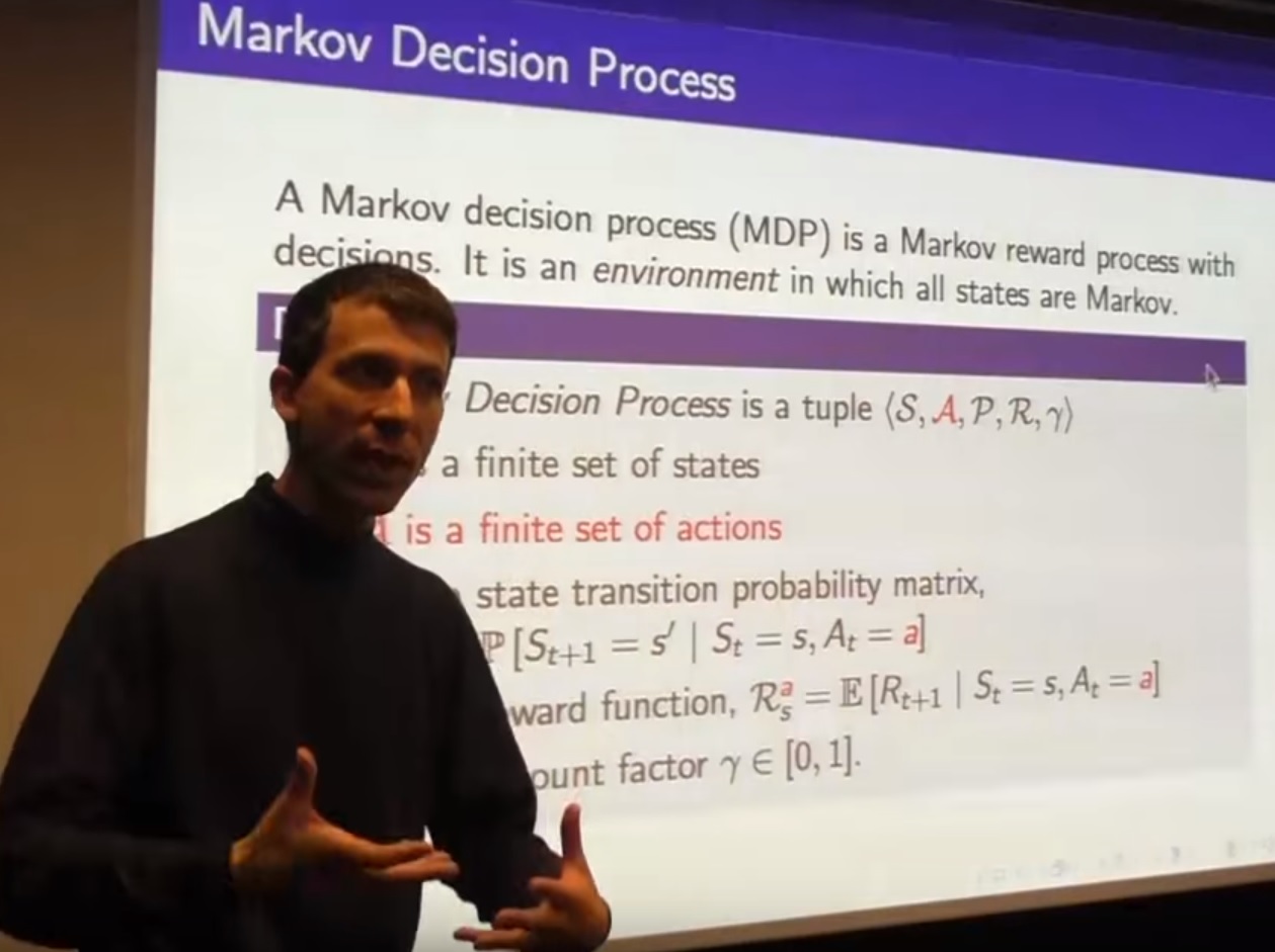
Lecture 2: Markov Decision Process

Markov processes:
- MDPs formally describe an environment for RL
- Almost all RL problems can be formalised as MDPs
- Def. Markov process: a random sequence of states with the Markov property, drawn from a distribution: [S,P] state space S and transition probability matrix P
- Good example: student markov chain (making it through a day at university) -> slide 8
Markov reward processes:
- It is a MP with value judgments (how good it is to be in a state): [S, P, R, gamma] with reward function R (immediate reward for being in a state) and discount factor
- In RL, we actually care about the total (cumulated, discounted) reward, called the return (or goal) G
- gamma is to quantify the present value of future rewards (i.e., because of uncertainty: now they are not yet fully sure, also because our model not being perfect; also because it is just mathematically convenient to do so)
- Value function: the long-term value of being in a state (the thing we care about in RL) V(s)=E[G_t|S_t=s] (expectation because we are not talking here about one concrete sample from the MRP, but about the stochastic process as a whole, i.e. the average over all possible episodes from s to the end)
- Great example -> slide 17
- Bellman equation for MRPs: to break up the value function into two parts: immediate reward R_{t+1} and discounted future reward gamma*v(S_{t+1})
- The Bellman euqation is not just for estimating the value function; it is an identity: every proper value function has to obey this decompositon into immediate reward and discounted averaged one-step look-ahead
Markov decision processes:
- MRP with decisions, i.e. we not just want to evaluate return, but maximize it: [S, A, P, R, gamma] with actions A
- What does it mean to make decisions? => policy (distribution over actions given states) completely defines an agent’s behaviour
- (Given an MDP and a fixed policy, the resulting sequence of states is a Markov process, and the state and reward sequence is an MRP)
- Given a policy, there are two types of value functions:
  - state-value function v_{pi}(s): how good is it to be in s if I am following pi
  - action-value function q_{pi}(s,a): how good is it to take action a in state s if following pi afterwards
- Bellman equations can be constructed exactly the same way as above for v_{pi} and q_{pi}: immediate reward plus particular value function of where you end up
- Bellman euqations for both need a 2-step lookahead: over the (stochastic) policy, and over the (stochastic) dynamics of the environment
What we really care about: finding the best behaviour in an MDP
- The optimal value function is the maximum v/q over all pi
- When you know q*, you are done: you have everything to behave optimally within your MDP -> the optimal policy follows directly from it
- There is always at least one deterministic optimal policy (greater or equal value v(s) for each s, compared to all other policies) -> we don’t need combinations of policies for doing well on different parts of the MDP
- How arrive at q*? Take Bellman equation for q and “work backwards” from terminal state
- (before we looked at Bellman expectation equations; what now follows are the Bellman optimality equations, or just “Bellman equations” in the literature)
- Here, we maximize over the actions we can choose, and average over where the process dynamics send us to (2-step lookahead)
- Bellman equations (in contrast to the version in MRPs) are non-linear (because of max) -> no direct solving through matrix inversion
- => need to solve iteratively (e.g. by dynamic programming: value or policy iteration)

Lecture 3: Planning by Dynamic Programming

Dynamic programming:
- Dynamic (it is about a sequence/temporal problem), programming (about optimizing a program/policy)
- Method: solve complex problems by divide&conquer
- Works if subproblems come up again and again, and their solution tells us something about the optimal overall solution (MDPs satisfy both properties, see Bellman equation [decomposition] and value function [cache for recurring solutions])
Planning:
- Prediction: not the full RL problem, but when we are given the full reward function + dynamics of system + policy -> output is the corresponding value function
- Control: no policy given -> output is optimal value function
- We care about control, so we use prediction as an inner loop to solve control
Policy evaluation: if I am given a policy, how good is it?
- Each iteration (synchronous update): update every state (we know the dynamics, it is planning!) in the value function using the Bellman expectation equation and the lookahead (just one step, not recursively!)
- Good example on slide 9/10: the value function helps us finding better policies (e.g., greedy according to the value function), even if it is created using a different policy (e.g., random)
Policy iteration: improve a given policy to get the best one
- How to improve a policy: 2 steps (a little related to EM)
  - Evaluate the policy (i.e., compute its value function)
  - Act greedily w.r.t. the computed value function
  - => will always converge to optimal policy (after usually many iterations)
- This works, because acting greedily for one step using the current q is at least as good (or better) than just following the current policy immediately -> see slide 19
- If it is only equally good, the current policy is already optimal
- Acting greedily doesn’t mean to greedily look for instantaneous rewards: we only (greedily) take the best current action and then look at the value function, which sums up all expected future rewards
- Policy evaluation has not to be done until convergence -> a few steps suffice to arrive at an estimate that will improve the policy in the next policy improvement step (if k=1, this is just called “value iteration” or “modified policy iteration”)
Value iteration (i.e., policy iteration with early stopping [just one iteration] on policy evaluation)
- This uses the Bellman optimality equation
- Intuition: think you have been told the optimal value of the states next to the goal state, and you are figuring out the other states’ values from there on backwards
- No explicit policy (intermediate value functions might not be achievable by any real policy, only in the end the policy will be optimal)
- Summary so far: -> slide 30 (using v instead of q so far is less complex, but only possible because we know the dynamics [it is still planning]; and doing value iteration is a simplification of policy iteration)
Extensions to make DP more practical
- Asynchronous backup: in each iteration, update just one state (saves computation and works as long as all states are still selected for update [in any order])
- Prioritised sweeping: in which order to update states? those first that change their value the most (as it has largest influence on result)
- Real-time DP: update only those states that a real agent using the current policy visits
- Biggest problem with DP are the full-width backups (consider all possible next actions and states) -> use sampling instead

Lecture 4: Model-Free Prediction

Introduction
- Last lecture was estimating/optimizing the value function of a known MDP; now we estimate for an unknown MDP (no dynamics / reward function given) -> from interaction (with environment) to value function
- Planning is model-based (dynamics given), RL is model-free (no one tells); prediction is evaluating a known policy, control is finding new policy
Monte-Carlo Learning
- Learn directly from complete episodes (i.e., update every state after the end of an episode)
- Basic idea: replace the expectation in v_{pi}(s)=E_{pi}[G_t|S_t=s] with the empirical mean
- Problem: how to deal with getting into a state we already have been in, again (to create several values to average over), and how to visit all states just from trajectories -> by following policy pi
- Blackjack example: only consider states with an interesting decision to make (i.e., do not learn actions for the sum of cards below 12, as you would always twist then as no risk is attached to it)
- Slide 11: axes of value function diagrams are two of the three values in the state; the third (usable ace) is displayed by the 2 rows of figures
TD Learning
- TD learns from incomplete episodes (i.e., online, “bootstrapping”) by replacing the return (used in the MC approach above after the episode run to the end) by the TD target (immediate reward plus discounted current estimate of v_s_{t+1})
- TD is superior to MC in several respects (e.g., more efficient, it has less variance but is biased); but TD does not always converge to v_{pi} when using function approximation
- MC converges to minimum MSE between estimated v and return; TD(0) converges to solution of maximum likelihood MDP that best fits the observed episodes (implicitly)
- TD(0) exploits the Markov property, thus it is more efficient in Markov environments (otherwise MC is more efficient)
TD(lambda): unification of Monte-Carlo and TD
- We can map all of RL on two axes: whether the algorithm does full backups vs. samples (i.e. averages over all possible actions/successor states [e.g., dynamic programming, exhaustive search]), or just uses samples (e.g., TD(0), MC), and whether backups are shallow (i.e., 1-step lookahead [e.g., TD(0)]) or deep (full trajectories [e.g., MC]) -> see Fig. 3 in survey paper by Arulkumaran et al., 2017
- lambda enables us to target the continuum on the “shallow/deep backups” axis
- The optimal lookahead depends on the problem, which is dissatisfactory; thus, the lambda-return averages all n-step returns, weighted by look-ahead (more look-ahead, less weight) -> slide 39
- TD(lambda) comes at the same computational cost as TD(0), thanks to the (memoryless) geometric weighting

Lecture 5: Model-Free Control

On-policy (learning on the job) vs. Off-policy (learning while following some else’s idea; looking over someone’s shoulder)
Last lecture: evaluate given policy in realistic setting; now: optimize it (find v*)
On-policy Monte-Carlo control
- General framework: generalised policy iteration -> slide 6
- 2 problems with just plugin in Monte Carlo simulation into this general framework: (1) it is not model-free (we need a model of the environment since we only have V, not Q); (2) we don’t explore if we always greedily follow the policy => so it would work with Q instead of V and acting epsilon-greedily instead of just greedily
- epsilon-greedy is guaranteed to improve (proven)
On-policy TD learning
- typical RL (here: with SARSA): it is slow in the beginning, but as soon as it learns something, it becomes faster and faster with doing better
Off-policy learning: e.g., for learning from human behaviour
- MC learning off policy doesn’t work -> have to use TD learning
- What works best off-policy (gets rid of importance sampling): Q-learning (as it is usually referred to) -> slide 36
Summary so far: TD methods are samples of the full updates done by DP methods -> slide 41

Lecture 6: Value Function Approximation

It is not supervised learning: iid training methods usually don’t work well because of the correlation in the samples of the same trajectory
Incremental prediction methods: do everything online, after each step in the environment (no collection of a larger “data set”)
- How “close” to optimum TD(0) with linear value function approximation converges depends on things like the discount factor -> slide 18
- In TD we are always pushing things to “later” because we trust in our estimate of later return
Incremental control methods: never converge to true q*, usually oscillate around it but come close
- In continuous control, you ofton don’t need to account for the differnces between maximum and minimum (say) acceleration -> so it becomes discrete again
- Bootstrapping (using lambda>0 in TD(lambda)) usually helps, need to find a sweet spot (lambda=1 usually is very bad)
- TD is not stable per se (isn’t guaranteed to converge) -> slide 30 shows when it is safe to use (for prediction), even when it practice it often works well
- For control, we basically have no guarantee that we will make progress (best case that it oscillates around the true q*)
Batch methods: gradient-based methods are not sample-efficient (don’t make best use of the data because of mini steps); gradient methods want to find best fit to all of the data
- Experience replay is an easy way to converge to the least squares solution over the complete data set of experience (that we didn’t have in the online case considered above)
- DQN is off-policy TD learning with non-linear function approximation -> it is anyhow stable because of experience replay and fixed (instead of non-stable, because of coming from a changing Q network) Q updates (by means of a fixed, saved few-thousand steps [hyperparameter!] older version of our Q network to which we bootstrap) that together hinder the convergence to diverge (“spiral out of control”)

Lecture 7: Policy Gradient Methods

Introduction: this is about working on (parameterize, then optimize) the policy directly, without putting the value function in the center (approximating it, then deriving the epsilon-greedy policy from it)
- Simplest method: policy gradient methods change the policy in the direction that makes it better
- Policy-based methods tend to be more stable (better convergence properties) and are especially good in continious or high-dimensional action spaces (because of the max() over actions in value-based methods like Q-learning or SARSA)
- Policy-based methods can learn a stochastic policy, that can find the goal much quicker if there is doubt (aliasing) about the state of the world (i.e., partial observability) -> slide 9
Monte-Carlo policy gradient
- The score function is a very familiar term from ML (maximum likelihood) and tells you in which direction to go to get “more” of something -> slide 16
- The whole point of the likelihood ratio trick is to get an expectation again for the gradient -> slide 19
- REINFORCE is the most straightforward approach to policy gradient
- MC policy gradient methods have nice learning curves but are very slow (very high variance because we plug in samples of the return [that vary a lot]) -> slide 22
Actor Critic methods: bring in a critic (estimate of value function) again to retain nice stability properties of policy gradient methods while reducing variance
Critic is built using methods from previous lectures for policy evaluation; then, the estimated Q is plugged into the gradient-of-objective-function equation
Q-AC is just an instance of generalised policy iteration, just with the gradient step instead of the epsilon-greedy improvement
Summary -> slide 41

Lecture 8: Integrating Learning and Planning

Introduction
- A model (in RL) is the agents understanding of the environment (1. state transitions; 2. how reward is given); that’s why building a model first is a 3rd way (besides value- and policy-based methods) to train an agent
- Advantage: can be efficiently trained by supervised learning (helps in evironments with complicated policies [sharp/tactically decisive decisions like in chess where one move can decide winning or loosing] like games that need lookahead) -> it is a more compact/useful representation of the environment
Model-based RL
- Sample-based planning: most simple yet powerful approach, uses learnt model only to sample simulated experience from it
- it helps because it breaks the curse of dimensionality (or rather branching factor for successive events): we sacrifice the detailed probabilities given by the learnt model and thus focus on the more likely stuff -> slide 18
- Slide 19: reasoning for our approach taken in the “Complexity 4.0” project & chapter (use a simulation model to learn an ML model)
- How to trade off learning the model vs. learning the “real thing” (value function/policy)? you act everytime you have to (gives real experience, used to build best model possible), then plan (simulate trajectories form model to improve q/pi) as long as you have time to think before you have to act again
Integrated architectures
- Dyna architecture does what was just proposed and is much more data efficient (w.r.t. real experience, as more data can be generated) already with 5 (and much more with 50) sampling (“thinking”) steps between 2 real observations -> slide 28
Simulation-based search
- Forward search: Key idea is to not explore the entire state space, but focus on what matters from the current state onwards (i.e., we only solve the sub-MDP starting from “now”)
- Simulation-based search: forward search using sample-based planning based on a model (i.e., not build/consider whole tree from now on, but sample trajectories, then apply model-free RL to them) -> slide 33
- Monte-Carlo tree search: search tree is built from scratch starting from current state and contains all states we visit in the course of action together with the actions we took, together with MC evaluations (q-values)
- MCTS process: repeat {evaluation (see above); improvement of tree (simulation) policy by methods from last lectures, e.g. epsilon-greedy} => this is just MC control (from previous lectures) applied to simulated experience -> slide 37
- MCTS converges to q*
- MCTS advantages: breaks “curse of dimensionality” by sampling; focuses on the “now” and the most likely successful actions through sampling; nice computational properties (parallelization, scaling, efficient)
- TD search has the advantage to potentially reduce the variance and being more efficient (than MC; more so if choosing lambda well), thanks to bootstrapping
- Recap on TD/MC: instead of waiting until the end of each simulated episode and taking the final reward to build up statistics of the value of our “now” state by taking the average (MC), we bootstrap a new estimate of the value of each intermediate state by means of current reward plus discounted expected reward according to current q estimate (TD)
- TD is especially effective in environments where states can be reached from many different paths (so that you already might to know something about the next state and have it encoded in your current q estimate) => so only difference between MC and TD search is in how we update our q values -> slide 51
- Slide 53: black is MCTS, blue is Dyna-2 (long-term memory from real experience, short-term memory from simulated experience)
- Final word: tree helps to focus “imagination” (planning) on the relevant part of the state/action space, and thus learning from simulation is highly effective

Lecture 9: Exploration and Exploitation

Exploration in multi-armed bandit problems
- Decaying epsilon-greedy is best exploration strategy, but depends on schedule (which depends on unknown optimal value function)
- Optimism in the face of uncertainty (uncertainty = fat tails of a distribution): if you have 3 distributions for e.g. reward, pick not from the one with the highest mean, but with the fattest tails towards the maximum; if those extend beyond the highest mean, this distribution has the highest potential to have an even higher mean when seeing more examples -> slide 15
- Upper Confidence Bound (UCB): select the action that maximizes the upper confidence bound on its q value (higher the more uncertainty we have, U_t(a) shrinks while we visit this action more often => it characterizes the “tail” from above) -> slide 17
- The UCB term helps us exploring without knowing more about the true q values except that they are bounded
- UCB vs. epsilon-greedy: UCB performs really well, epsilon-greedy can to this to but can be a disaster for wrong epsilon -> slide 21
- If you have prior knowledge about the bandit problem, you can use Thompson sampling, which can be shown to be asymptotically optimal (but is still, as UCB, a heuristic) -> slide 25
- UCB (and other “optimism in the face of uncertainty” methods like Thompson) will explore forever (accumulating lots of unnecessary regret) in case of huge/infinite action spaces, and don’t allow save exploration
Back to MDPs
- UCB is not quite optimal for full MDPs as we have uncertainty about our current q-values in two ways (1. because we haven’t seen enough examples yet in evaluation; 2. because we haven’t improved enough yet), and it is hard to account for both with U_t(a) -> slide 42 (not same as in video)

Lecture 10: Classic Games

(For a corrected video with visible slides, see here.)

Game theory:
- We have done our job if we found a RL policy that is a Nash equilibrium (in the context of RL: a joint policy for all players such that every player’s policy is a best response) -> it is the best overall policy, but not necessarily the best against a very specific opponent’s policy
- In self-play, the best response is solution to single-agent RL (where all other players are treated as part of the environment)
- If we can solve playing a game (by adapting to the environment dynamically created by the other players trhough self-play) and converge to a fixed point (i.e., all other players declare they found an optimal policy in return), we have found a nash equilibrium -> slide 7
- Two-player zero-sum game (perfect information): equal and opposite rewards for each player; a minimax policy (that ahieves max value for white and minimum for black) is a Nash equilibrium
Self-play RL:
- Search is very important in successin games, intuitively so because it helps formuing tactics for the concrete current situation the player is in
- Self-play RL, we always play (and improve the policy) for both players (minimax), and all the previous machinery applies (MC, TD variants) -> slide 20
- Logitello: tree search to come up with good moves in self-play was crucial (then used generalised policy iteration with MC evaluation of self-play games)
- TD Gammon: binary state vector had separate feature for each possible number of stones of each color in each position (i.e., one-hot encoded -> then neural network as value function approximator and TD(lambda) with greedy policy improvement without exploration [worked without exploration because of the stochasticity introduced by the dice that helps in anyhow seeing a lot of the state space])
Combining RL and minimax search:
- TD Root (A. Samuel’s Checkers): backup value of s_t not from v(s_{t+1}), but from the result of a tree search on s_{t+1} (first ever TD algorithm)
- TD Leaf: update also the decisive leaf node and the rest of its branch (not just the root) in the tree of the search on s_t with the “winning” node’s value in the minimax search of s_{t+1}
- TreeStrap: different from TD Leaf, this is also effective in self play and from random weights (works by updating/learning to predict any value in the search tree; this doesn’t mix the backup from search with the backup from randomly searching as previous ideas did and which is not effective)
RL in imperfect information games:
- Naively applying MCTS/UCT etc. (that are so effective in fully observable games like Go) to games of imperfect information usually “blows up”/diverges
- Need a search tree per player built by smooth-UCT search (that remembers the average policy of the opponent by counting avery action they ever played during self-play)
Games & RL - a recipe:
- v: often binary linear, in future more NN
- RL: TD(lambda) with self-play and search (crucial, for tactics)

Written on August 27, 2018 (last modified: August 27, 2018)